Flash spectrum videos have been successfully used to estimate the solar radius JOA2022_2.pdf (iota-es.de) and the same methodology offers the possibility to probe the distribution of elements in the chromosphere.
During a total solar eclipse, when the photosphere disappears below a lunar valley, the light of the chromosphere becomes predominant and studying the spectrum of its light allows the analysis of the different elements present in the lowermost layers of the Sun’s atmosphere.
Moreover, the more the photosphere descend below the lunar valley, the more layers of this atmosphere is covered. So the evolution of the spectrum intensity over time can be translated into a sampling that informs us on the distributions of the elements as a functions of their height over the photosphere.
This technique has been used since the early 1900’s 1947ApJ…105….1M (harvard.edu), and more recently by Voulgaris et. al. 1202.1535.pdf (arxiv.org) with greater spectral resolution
In our setup, a Canon EOS 6D with a Canon EF 70–200 mm f/4L USM lens, recorded a video, with exposure of 1/60 s at ISO 100, of the flash spectrum generated by a diffraction grating, etched with 235 lines/mm mounted in front of the lens, during the Aug 21,2017 Total Solar Eclipse in Oregon, at the edge of the umbral shadow path (117° 13′ 0,9″.8 W, 43° 57′ 10″.9 N).
The flash spectrum is extracted from the video by considering the light coming from a single Baily’s bead. The light intensity extracted from the video is converted into linearised luminance Y by removing the gamma correction. The timing of each frame is determined by simulation (more details can be found in Appendix A of https://iopscience.iop.org/article/10.3847/1538-4365/ac1279/meta), and it is estimated to have an uncertainty of ca. 0.15s.
The video shows
– on top left: the video of the flash spectrum and the sampling line in green, where the flash spectrum has been measured for the specific bead generated by the lunar valley indicated by the green arrow,
– on top right: the flash spectrum, measured as the luminance along the sampling line with some peaks annotated with the element generating it,
– on bottom right: in black the lunar limb profile and in red the Sun profile descending beow the valley of the indicated bead,
– on bottom right: the intensity of some peaks as a function of the height over the photosphere
The intensity of a peak over time can be converted to the intensity as a function of the height over the photosphere. This transformation is obtain by leveraging the computational model described here.
We can give a numerical example. Let’s assume that the solar radius is 959.95″ (at 1au), which is equivalent to 696220km. This is the assumed radius of the photosphere. The computational model tells us that the time of contact of the photosphere with the bottom of the lunar valley generating the Baily’s bead happens at 17h 25m 25.8s UTC. Let’s now consider a layer 0.2″ above the photosphere, that is to say a layer at a radius of 960.15″, equivalent to 696370km. The time of contact of this shell is 17h 25m 26.7s UTC. Let’s now consider a layer 0.4″ above the photosphere, that is to say a layer at a radius of 960.35″, equivalent to 696510km. The time of contact of this shell is 17h 25m 27.7s UTC.
At time 17h 25m 25.8s UTC, the intensity of the light in the spectrum is coming for all the layers of the solar atmosphere, from the edge of the photosphere and above. At time 17h 25m 26.7s UTC, the lowermost (696370 – 696220)km = 150km of the solar atmosphere are already below the bottom of the lunar valley, so the intensity of the light is only representative of the layers 150km above the photosphere and higher. At time 17h 25m 27.7s UTC, only the layers (696510 – 696220)km = 290km above the photosphere and higher contribute.
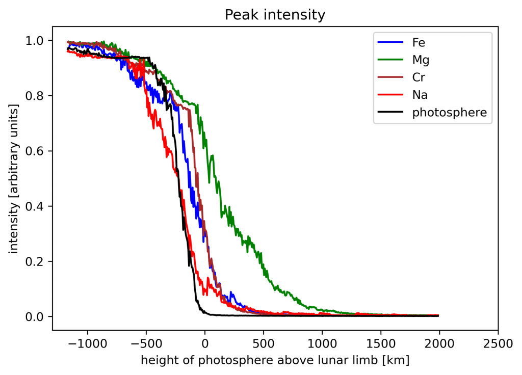
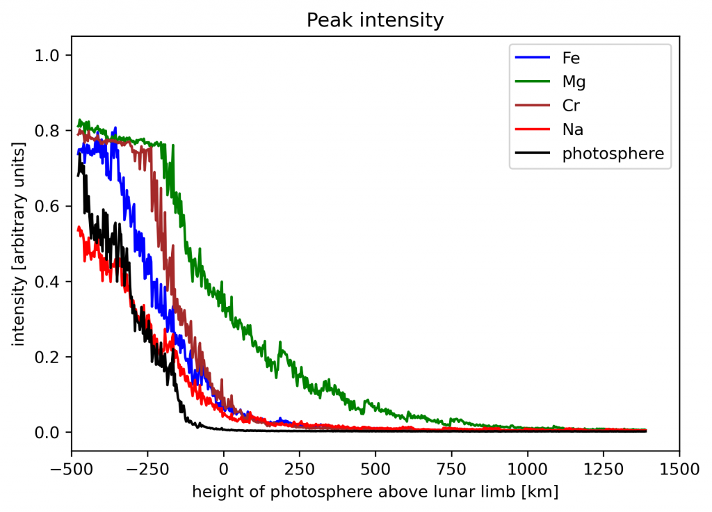
The analysis shows that Iron and Chromium are present in detectable quantities from the edge of the photosphere up to about 5-700km. Sodium, at least traces of it, is present up to 1000km above the photosphere. Magnesium goes up to about 1500km. Helium and Hydrogen are of course also present in the lowermost layers of the solar atmosphere but they extend out to many thousands of kilometers. Ours is a simple analysis but it shows that various elements are not equally distributed in the solar atmosphere and it allows estimating the regions where they are found in detectable quantity.
The intensity of the emission of the various elements as a function of the height over the photosphere can be performed considering other Baily’s beads. Different beads are generated by very different part of the Sun limb and in principle could show some variability on the density of the elements over altitude. The following plots show the result of the analysis for two different Baily’s beads. The results show some variability but they are not too dissimilar.